AI Notes - Machine Learning
Artificial Intelligence - Machine Learning
The foundation of artificial intelligence is machine learning. As the name suggests, it lets machines process data and learn from that data so they can make decisions on their own. Put simply, machine learning lets a machine learn and improve without being explicitly programmed for the task.
Machine learning falls broadly into three kinds: supervised learning, unsupervised learning, and deep learning.
Supervised Learning
Supervised learning is a machine learning approach that learns a model or function from labeled training data (that is, known inputs and outputs). The model or function can then be used to predict new, unseen data. During training, whenever the model's prediction differs from the actual result, the model is adjusted to reduce that difference. It is as if a "supervisor" were guiding the machine on how to learn.
Supervised learning naturally depends on training algorithms. Its defining characteristic is that it needs both inputs and outputs, with feedback on the output (and the data used in supervised learning is always labeled).
Common supervised learning algorithms include linear regression, logistic regression, decision trees, support vector machines (SVM), and the K-NN (nearest neighbor) algorithm.
Linear Regression
Linear regression is a common predictive analysis method, suitable when two or more variables have a linear relationship. In machine learning, the goal of linear regression is to find a best-fit line that minimizes the sum of the vertical distances (the errors) from all data points to that line. This process is also known as the least squares method.
The general form of a linear regression model is Y = aX + b, where Y is the dependent variable (the target we want to predict), X is the independent variable (the input we use to predict), and a and b are model parameters that determine the slope and intercept of the line.
Linear regression provides a way to quantify the relationship between independent and dependent variables, and it underpins many more complex models and techniques. It is widely used across fields including economics, biology, environmental science, and the social sciences.
Here is an example:
import numpy as np
import matplotlib.pyplot as plt

from sklearn.linear_model import LinearRegression

def f(x):
    np.random.seed(42)
    y = 0.1 * x + 1.25 + 0.2 * np.random.randn(x.shape[0])
    return y

x = np.arange(0, 20, 0.5)
y = f(x)

plt.scatter(x, y, label='Actual Data', color='blue')
plt.title('Data')
plt.legend()
The code above generates a set of scattered points representing a series of observed events, as shown:
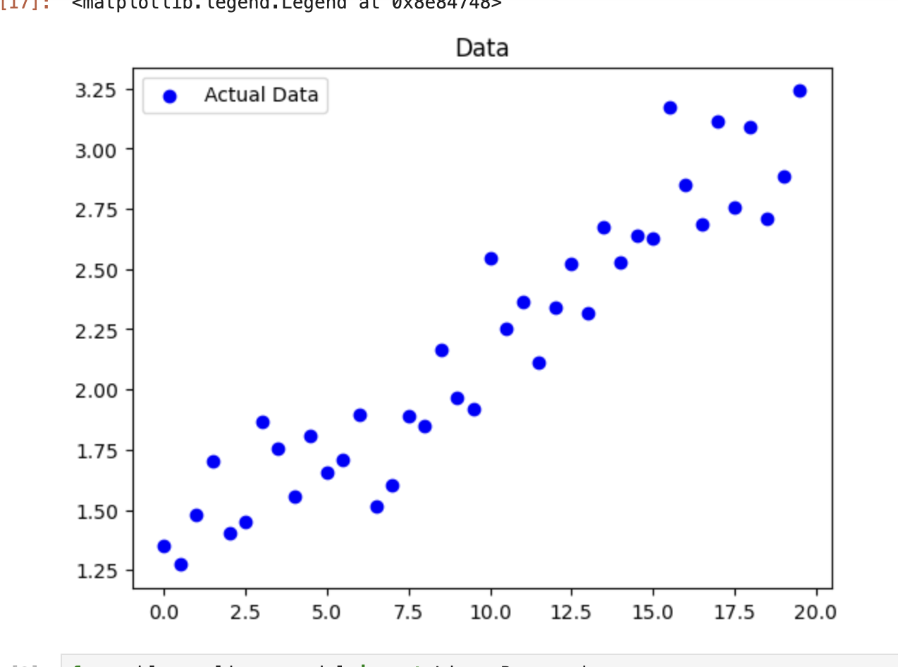
With that, the sample data is ready.
Next comes model training. We use the linear regression algorithm from the machine learning library and train the model (printing the slope coefficient and intercept):
from sklearn.linear_model import LinearRegression

regression_lineal = LinearRegression()
regression_lineal.fit(x.reshape(-1, 1), y)

print('w = ' + str(regression_lineal.coef_) + ', b = ' + str(regression_lineal.intercept_))
w = [0.09183522], b = 1.2858792525736682
Then we make a prediction (the input here is 5, which is close to the points in the plot):
new_x = np.array([5])
prediction = regression_lineal.predict(new_x.reshape(-1, 1))
print(prediction)
[1.74505534]
We can also compute evaluation metrics for the model. Here the standard deviation and R2 are computed:
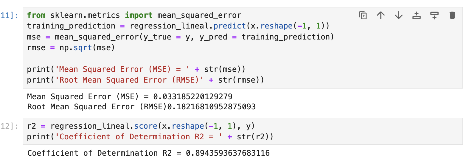
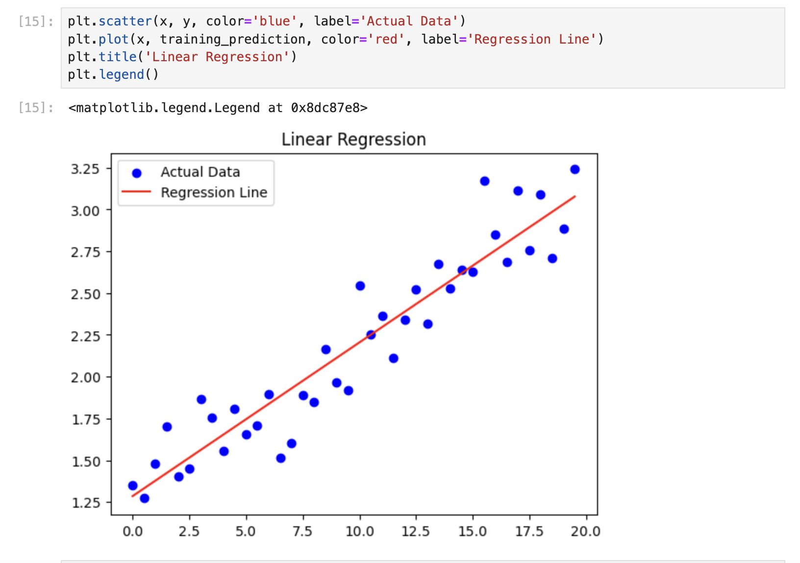
The score is close to 0.9, which indicates a reasonably good fit. Finally, here is the fitted line:
Logistic Regression
Logistic regression is a statistical technique for predictive analysis used to solve binary classification problems. It uses the logistic function to map the output of a linear regression into the range between 0 and 1, which makes it a good tool for classification. The main goal of logistic regression is to find the logistic function that best describes the relationship between the input variables and the output; the function's output can be interpreted as the probability that an event occurs.
The general form of a logistic regression model is p = 1 / (1 + e^(-z)), where p is the predicted probability, z = aX + b, a and b are model parameters, and X is the input variable. During training we need to find the a and b that minimize the difference between the predicted probabilities and the actual class labels. This is usually done with maximum likelihood estimation or gradient descent.
Logistic regression is very useful for understanding the factors that influence an outcome, predicting outcomes, and building simple classification models. It is widely used in finance, healthcare, the social sciences, and many other fields.
Decision Trees
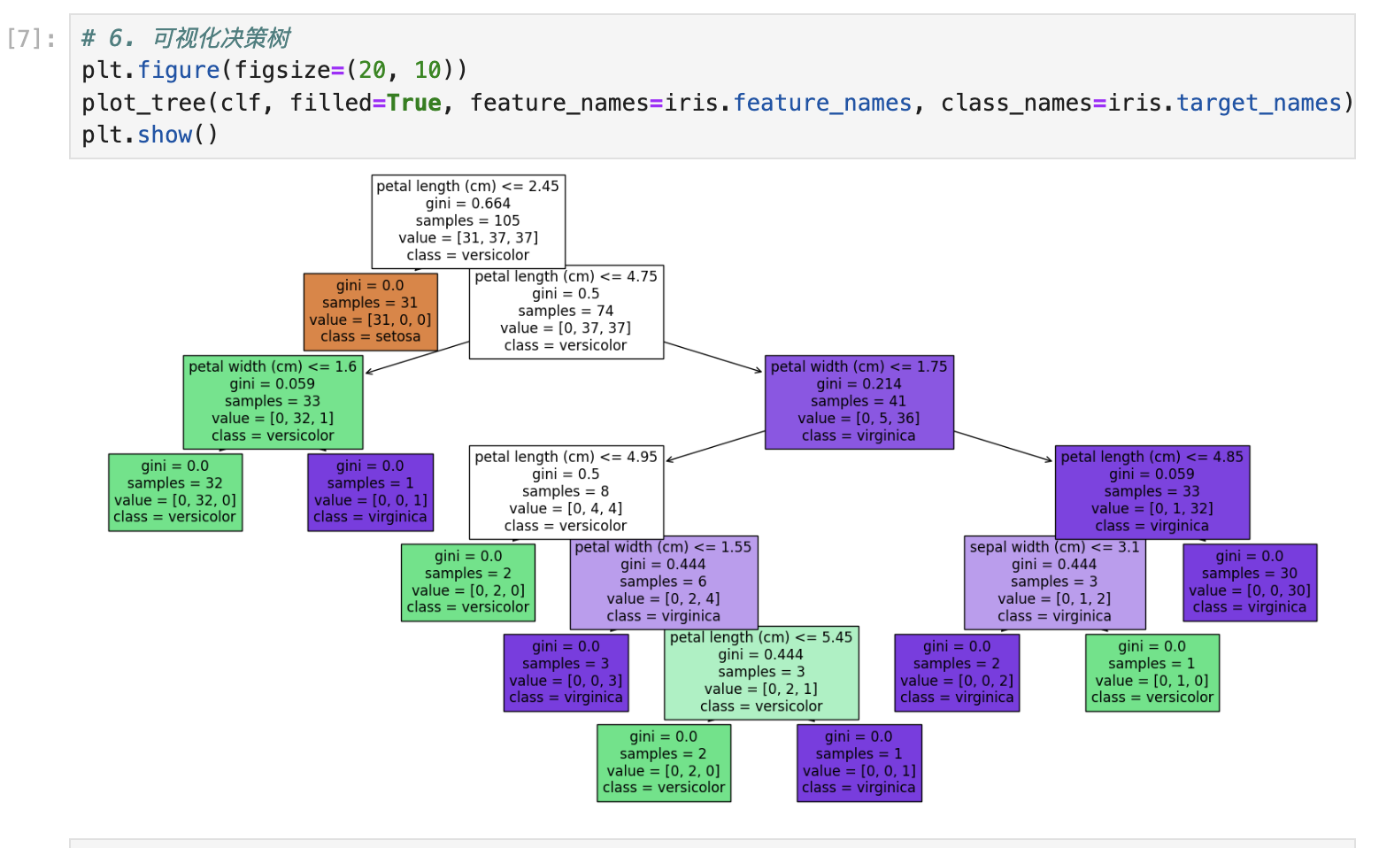
A decision tree is a tree-structured machine learning model for classification and regression. It splits the dataset into different subsets through a series of splitting rules, eventually forming a tree: each node represents a feature, each branch represents a possible value of that feature, and each leaf represents a classification or regression result.
The main advantages of decision trees are:
- Easy to understand and interpret: The model's structure is intuitive, easy to explain, and well suited to visualization.
- Little data preprocessing: Decision trees do not need much preprocessing, such as normalization or filling in missing values.
- Handles multiple data types: Decision trees can handle both numerical and categorical data, which makes them quite flexible.
Building a decision tree usually involves these steps:
- Choose the best feature: Select the best feature to split on according to some metric (such as information gain or the Gini index).
- Create split points: Create split points based on the chosen feature, dividing the data into several subsets.
- Split recursively: Repeat steps 1 and 2 recursively on each subset until a stopping condition is met (such as reaching the maximum tree depth, or the number of samples in a leaf falling below a threshold).
The disadvantages of decision trees are:
- Prone to overfitting: Decision trees easily overfit the training data, especially when the tree is deep. Pruning or setting a maximum depth can mitigate this.
- Sensitive to noise: Decision trees are fairly sensitive to noisy data, which can make the tree unstable.
Decision trees perform well in many practical applications, such as credit scoring, medical diagnosis, and market analysis. They can also be combined with other models, as in ensemble methods like random forests and gradient boosted trees.
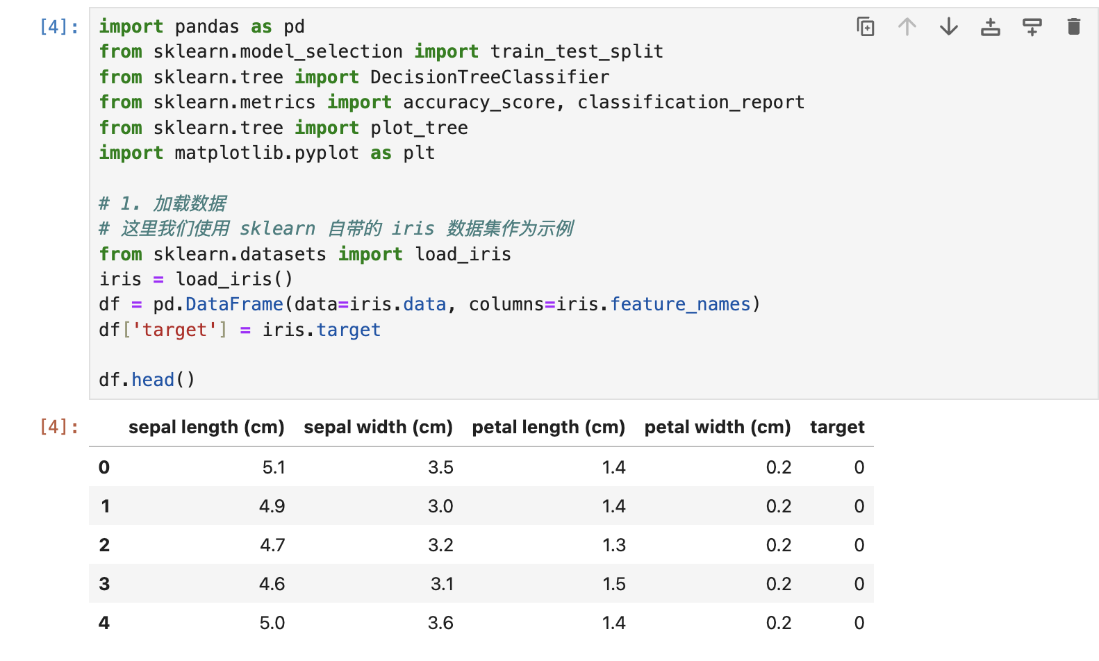
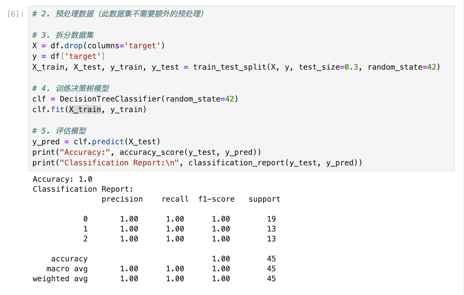
Here is a simple decision tree classification example:
K-NN (Nearest Neighbor) Algorithm
The K-NN algorithm, short for K-Nearest Neighbors, is a simple and intuitive method for classification and regression. Its basic idea is: given a sample to classify, find the K samples in the training set closest to it, then decide the sample's class from those K samples by voting or averaging.
The steps of K-NN are:
- Choose K: Pick a positive integer K, the number of nearest neighbors to consider.
- Compute distances: For the sample to classify, compute its distance to every sample in the training set. Common distance metrics include Euclidean distance and Manhattan distance.
- Select the K nearest neighbors: Based on the computed distances, pick the K closest samples from the training set.
- Vote or average: Let the K nearest neighbors vote and assign the most frequent class to the sample; for regression, use the average of the K nearest neighbors as the prediction.
Advantages of K-NN:
- Simple to implement: K-NN has no explicit training phase; it classifies and regresses directly based on distance.
- Non-parametric model: K-NN does not need to learn model parameters, which suits small training sets.
Disadvantages of K-NN:
- Computationally expensive: For every sample to classify, distances to all training samples must be computed, which is costly.
- Poor on high-dimensional data: In high-dimensional spaces, distances between data points become hard to measure meaningfully, and K-NN performs poorly.
- Sensitive to noise: K-NN is fairly sensitive to noise and outliers, which affects classification results.
Even so, K-NN still performs well in many practical applications, especially classification problems—for example, handwritten digit recognition, image classification, and text classification.
Unsupervised Learning
Unsupervised learning is a machine learning approach that does not use labeled data during training. It lets the algorithm learn from the input data by itself and identify patterns and structure within it. The goal is usually to uncover patterns or relationships hidden in the data, such as through clustering or dimensionality reduction. Because there is no predefined target or output variable, unsupervised learning is often used for exploratory analysis to help researchers identify unknown patterns or relationships.
Its typical characteristic is that there is input data but no output data (unsupervised learning uses unlabeled data).
In unsupervised learning, the input data is unstructured. To handle this unlabeled, unstructured data, it needs to be clustered and reduced in dimension so that useful information can be extracted.
Common unsupervised algorithms include clustering algorithms (K-means) and principal component analysis (PCA).
K-means Algorithm
K-means is a common unsupervised learning algorithm used to partition a dataset into K clusters. It works by iterative optimization, assigning data points to the nearest cluster center, so that similarity within each cluster is maximized and similarity between clusters is minimized. The steps are:
- Randomly choose K initial cluster centers.
- Assign each data point to the nearest cluster center.
- Compute the new center of each cluster, i.e., the mean of all data points in the cluster.
- Repeat steps 2 and 3 until the cluster centers no longer change significantly or a preset number of iterations is reached.
K-means is simple and efficient and works for large datasets, but K must be specified in advance, and the algorithm is fairly sensitive to the choice of initial cluster centers.
Principal Component Analysis (PCA)
Principal component analysis (PCA) is a statistical method that simplifies a dataset through dimensionality reduction. Its purpose is to find the lower-dimensional space that best represents the distribution of the original data. PCA works by creating a new coordinate system and remapping the original data onto it. The basis of the new coordinate system consists of the principal components of the original data (the directions of greatest variance). In the new system, most of the information is compressed into the first principal component, the next largest share into the second, and so on. By keeping the first few principal components and discarding the rest, we reduce the data's dimensionality. PCA is widely used in image compression, data visualization, noise filtering, feature extraction, and data preprocessing.
Deep Learning
Deep learning is a machine learning approach that tries to mimic how the human brain works: by training on large amounts of data, a computer model learns to recognize patterns and make high-level decisions. At the core of deep learning are neural networks, especially deep neural networks, which contain multiple hidden layers, each performing a specific kind of data processing. Deep learning is widely used in speech recognition, image recognition, natural language processing, and other fields, where it has delivered significant results.