Hands-On Linear Regression Training with PyTorch
Based on Jupyter Notebook examples from my own experiments, this post uses PyTorch to build, train, and understand a linear regression model from scratch. It is aimed at beginners, and also helps you form an accurate mental model of PyTorch's autograd and training loop.
1. Recap: the linear regression problem
Linear regression is the most basic supervised learning model. Its mathematical form is:
where:
- : input feature
- : weight
- : bias
- : predicted value
The goal of training is to learn suitable , from the data so that the prediction is as close as possible to the true value .
2. PyTorch basics: Tensors and autograd
What is a Tensor
In a Jupyter Notebook environment, install torch first, then create a sample tensor:
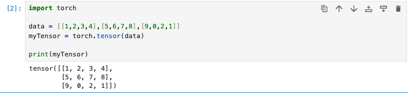
This is the simplest kind of Tensor: it has no gradient and is constructed from a matrix-like array. A Tensor has several important attributes, including shape, dtype, and device.
shape: the shape of the matrix, i.e. how many rows and columns.dtype: the data type of the elements.device: the device the tensor lives on, typicallycpuorcuda.
A
deviceofcudaenables NVIDIA's CUDA, running computation on the GPU, which can significantly speed up tensor operations.
Example:
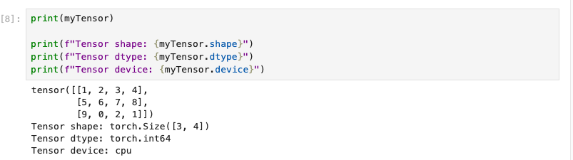
So a Tensor is essentially a wrapper around matrix data. Let's explore its other features.
Autograd on Tensors
Having looked at creating Tensors and their attributes, next comes a parameter you will use in any ML/LLM work: requires_grad. It is the core of creating tensors that support automatic differentiation:
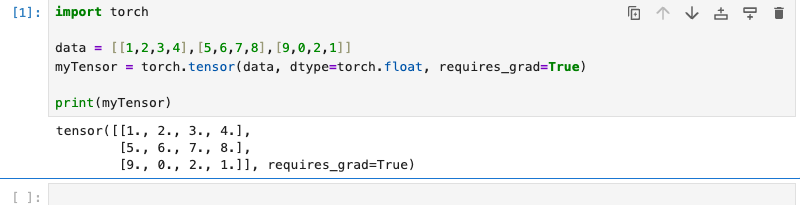
requires_grad means that computations involving the Tensor are tracked, so that you can later differentiate with respect to it (compute gradients).
In the example below, we first run a series of computations on Tensors:
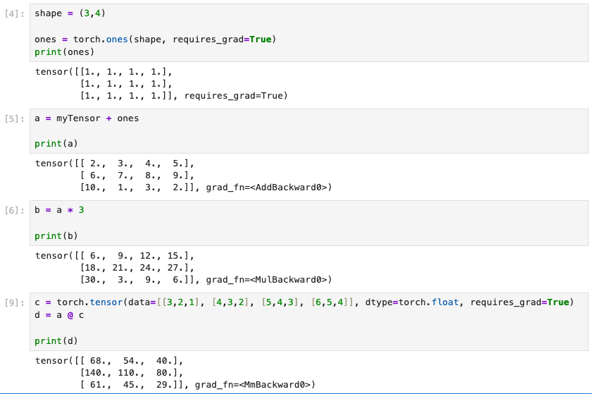
You can see that the Tensors a, b, c, and d all have a grad_fn attribute, which indicates the operation that produced that Tensor.
Backpropagation on Tensors
Tensor backpropagation provides the ability to trace computations, but backward() can only be called directly on a scalar.
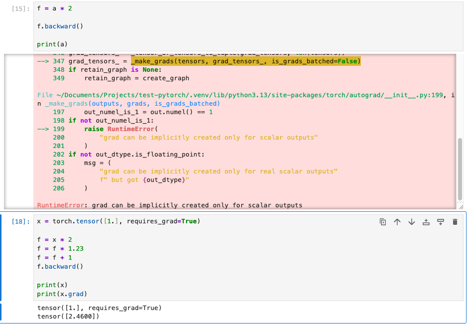
As shown above, the scalar x goes through a series of computations, and in the end its gradient (slope) can be read from the .grad attribute.
Besides what is covered here, Tensors also support median, max, sum, and much more; see the official documentation for details.
3. Building a linear layer with torch.nn.Linear
Here we use the linear model from torch's Neural Network module; the core is building a basic linear layer:
linear_layer = torch.nn.Linear(in_features=1, out_features=1)

print(linear_layer.weight)
print(linear_layer.bias)
This step is equivalent to defining the formula:
where:
weightcorresponds tobiascorresponds to
4. Defining the linear regression model
Defining the linear regression model takes several steps.
Step 1: Prepare the data
The data here generates X in the formula with random numbers, then applies the basic computation plus a bit of random noise to simulate a real-world environment.
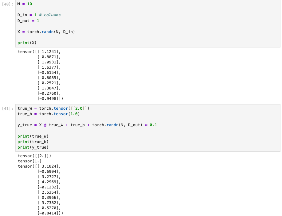
Here true_W and true_b are the ground-truth values and y_true is the simulated output. Through training, we want to find W and b close to the ground truth.
In a real scenario,
Xmight be an instrument's input (the independent variable), andy_truethe historically recorded results for eachX(the dependent variable). This data is what the model is trained on, and in practice it would be much larger.
Step 2: Define the regression model
There is more than one way to implement this. Although defining a model by subclassing torch.nn.Module is generally recommended, to illustrate what happens inside, I use a functional style here and compute the parameter updates by hand.
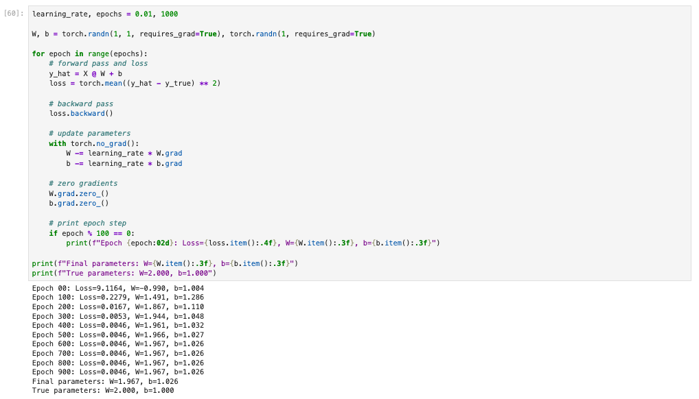
Just this one loop is all it takes to train the model.
5. Forward pass
What is the forward pass
The forward pass feeds input data through the model to produce predictions.
input data → model → predicted result
(That is: input data → model → predictions.)
The model here starts out inaccurate, so its outputs may be wrong; the parameters need further adjustment to improve accuracy.
The corresponding code
Here is the code:
# forward pass and loss
y_hat = X @ W + b
PyTorch automatically builds the computation graph here and records the relationships between operations (see the Tensor section above).
6. Defining the loss function
The most common loss for linear regression is mean squared error (MSE):
loss = torch.mean((y_hat - y_true) ** 2)
Mathematically:
The loss measures how good the model's predictions are; the smaller, the better.
7. Backward pass
What is the backward pass
During the forward pass, a computation graph is built and the relationships between operations are recorded. The backward pass propagates in the opposite direction along that graph, computing the gradients of every parameter with requires_grad=True.
The corresponding code
The backward pass is just one line:
# backward pass
loss.backward()
With this single call, we can compute the gradients of our two parameters, W and b.
8. Updating the parameters
The core snippet for updating parameters:
# update parameters
with torch.no_grad():
    W -= learning_rate * W.grad
    b -= learning_rate * b.grad

# zero gradients
W.grad.zero_()
b.grad.zero_()
Here we nudge the parameters to reduce the loss above, so that W and b approach their ground-truth values.
Two things to note:
- So that adjusting
Wandbdoes not get recorded in the computation graph, we usetorch.no_grad; inside it, tensor operations are not recorded in the graph. - After updating the parameters, we need to reset the gradients of
Wandb; otherwise they accumulate into the next iteration and cause confusion.
9. A more idiomatic approach
In real-world settings, training code is not usually written like this. With two parameters you can do it by hand, but LLMs have 7B, 256B, or more parameters, so writing it this way is completely impractical. torch already provides ready-made implementations of the manual computation above, and much more besides. Below is a more general approach (defining the model by subclassing torch.nn.Module and using torch's built-in machinery).
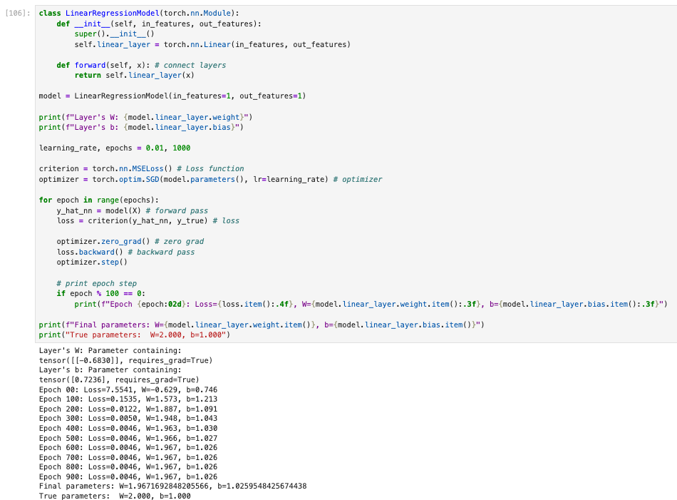
Because torch already defines the common models, optimizers, and loss functions, following this conventional style hides all of the parameter-update logic inside the optimizer, which is very clean.
10. Summary
Through the hands-on example in this post, we started from the most basic mathematical model, walked through the entire process of training a linear regression model in PyTorch, and gradually opened up the "black box" of PyTorch's autograd and training mechanics.
The key takeaways:
-
Linear regression is not complicated at its core Whether it is the mathematical formula
or PyTorch's
nn.Linear, both are essentially an engineered wrapper around this one formula. Understanding that helps you keep your "model intuition" as you move on to more complex models. -
The Tensor is PyTorch's core data structure A Tensor is more than a "multi-dimensional array": with
requires_grad=True, it becomes a node in the computation graph and automatically participates in gradient computation, which is the foundation of PyTorch's efficient training. -
Forward and backward form the training loop
- Forward pass: compute predictions and loss from the current parameters
- Backward pass: compute gradients by propagating the loss backward
- Parameter update: use the gradients to update the parameters
This flow applies not only to linear regression but to almost every deep learning model.
-
Understanding a hand-written training loop matters Although in practice we usually use:
nn.Moduletorch.optimnn.MSELoss
implementing parameter updates and gradient zeroing by hand lets you truly understand:
- where gradients come from
- why you need
zero_grad() - why parameter updates belong inside
torch.no_grad()
-
High-level abstractions are built on low-level principles PyTorch's high-level APIs are not "magic"; they are a high-level abstraction over these basic steps. Once you understand the underlying logic, the standard style turns out to be both elegant and reliable.
Overall, linear regression is the best starting point for learning PyTorch and deep learning. If you truly understand every step in this post, then multi-layer networks, CNNs, RNNs, and today's popular large language models (LLMs) all share the same training lineage.
Directions you can try next:
- Use real datasets (e.g. house prices, time series)
- Introduce
Dataset/DataLoader - Move the model to the GPU (CUDA)
- Extend to multi-dimensional features or multi-layer networks
Understand the fundamentals, and you can go much further.